Technical Analysis of School Bus Routing Software

I wrote this piece because every vendor says "we use AI" and almost none of them will tell you what that means in practice. When we were building RouteBot's solver, the first version looked great on small test sets and fell apart on a real district — 800 students, three schools, mixed SPED fleet. The assignment was fine; the sequencing was fine; together they produced routes that backtracked through the same intersection four times because the clustering ignored directional coherence. We rewrote the loop, and that lesson shaped how I think about the whole stack.

This is the technical companion to our Complete Guide to School Bus Routing Software. That piece covers the business case — when to switch, what changes, and why it matters. This one goes under the hood: the optimization framework, the constraint types that break naive implementations, and the metrics you should track to know whether the system is actually doing its job.

If you are a transportation planner evaluating products, this will help you ask better questions. If you are an engineer or operations researcher, this is how we think about the problem at RouteBot.

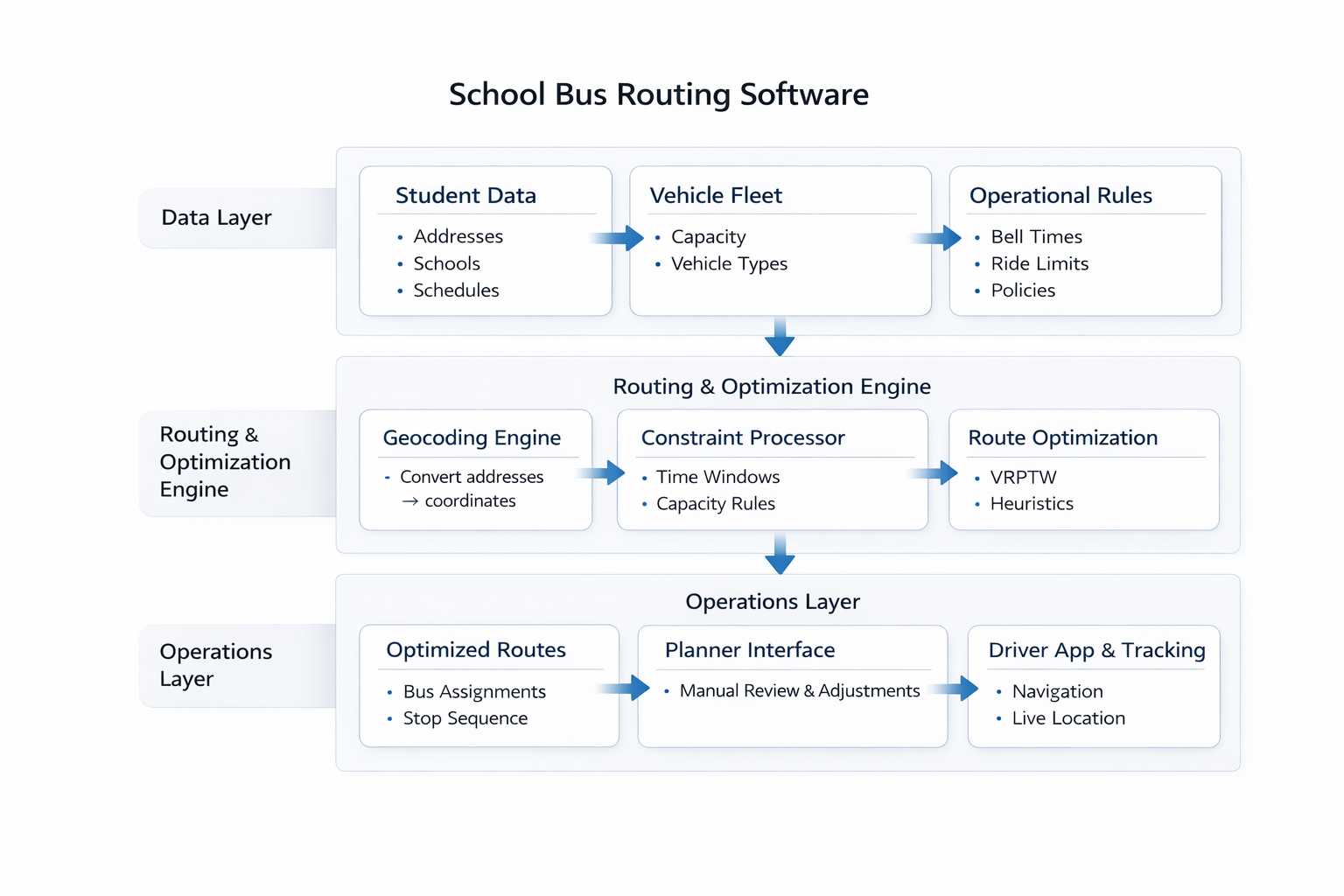
Student data, fleet constraints, and operational rules feed into an optimization engine. The engine proposes routes; planners and drivers review before anything goes live.

The Vehicle Routing Problem, school bus edition

Every school bus routing product is, at its core, solving a variant of the Vehicle Routing Problem (VRP). The textbook formulation is clean: given a set of customers, a fleet of vehicles, and a cost function, find the assignment and visit order that minimizes total cost. In practice it's a mess — because schools introduce constraints that generic freight routing doesn't care about.

School bus routing specifically maps to VRPTW — VRP with Time Windows. Each stop has a window in which service must begin (pickup between 7:10 and 7:25 AM, say). Miss the window and the route is infeasible.

The "cost" being minimized is usually some weighted combination of:

Total fleet size (buses in service)
Total route miles or drive time
Total deadhead (empty repositioning)

These objectives often conflict. You can reduce bus count by cramming more stops onto fewer routes, but that drives up per-route distance and ride time. The optimizer has to balance them, and the weights reflect policy as much as math.

What makes VRPTW hard

VRP is NP-hard, which in plain terms means there's no known algorithm that solves it efficiently at scale. A 15-stop route has 1,307,674,368,000 possible orderings. Add time windows, mixed capacities, and multiple depots, and exact solutions become computationally impractical beyond small instances.

This is why every production-grade school bus router uses heuristics or metaheuristics rather than exact solvers. You give up the guarantee of mathematical optimality in exchange for solutions that are very good — typically within 1–5% of the theoretical best — in runtime measured in minutes, not centuries.

The two optimization layers

In practice the problem decomposes into two linked subproblems. Most systems treat them as a loop rather than a strict pipeline: the assignment layer feeds the routing layer, the routing layer's costs feed back to reassignment, and the system iterates until improvements stop.

Layer 1: Clustering and assignment

Which students ride which bus?

The algorithm clusters students by geographic proximity and time-window compatibility, then assigns clusters to vehicles while respecting capacity. This isn't simple proximity grouping — it needs to consider:

Directional coherence. Students in the same area but in opposite directions from the school shouldn't necessarily share a bus, because the resulting route would double back on itself.
Capacity vectors. A bus isn't just "44 seats." It might be 40 general seats + 2 wheelchair securements + 1 aide position. A student needing a wheelchair slot can only go on a vehicle that has one open.
Time-window feasibility. Two clusters might be geographically close but temporally incompatible — one needs pickup at 7:10, the other at 7:40, and a single bus can't serve both within windows.

The counterintuitive result: sometimes swapping a handful of students between two buses shaves more mileage than resequencing every stop on one of them. The biggest efficiency gains often come from reassignment, not from routing tweaks within a fixed assignment.

Layer 2: Stop sequencing

Given the students on a bus, what order should it visit their stops?

This is a constrained Traveling Salesman Problem (TSP). The optimizer finds the stop order that minimizes drive time while respecting pickup windows. In a school context you're typically working with real road networks — actual turn penalties, one-way streets, seasonal road closures — not straight-line distances.

For a real-world district with hundreds of routes, even the TSP layer alone would be intractable if solved exactly. Heuristics dominate here too: nearest-neighbor initialization followed by local search improvements like 2-opt, Or-opt, or more aggressive neighborhood moves.

Constraint modeling: where theory hits pavement

The difference between routing software that works in a demo and routing software that survives September is constraint modeling. Here's what actually matters.

Hard constraints (never violated)

Vehicle capacity. Including differentiated capacities — general seats, wheelchair positions, special equipment. If the model treats every seat as identical, SPED routing collapses.

Bell times and pickup windows. The school's start time is not negotiable. Pickup windows derived from it are hard boundaries. A route that arrives 2 minutes late isn't "close enough" — it's infeasible.

Vehicle-student compatibility. A student who requires a lift-equipped bus cannot be assigned to a standard vehicle. This sounds obvious but requires the data model to carry vehicle-type attributes and match them against student requirements.

Maximum route duration. Many districts have policy or regulatory limits on how long a student can be on the bus. This constrains both assignment and sequencing: you can't serve too many stops on one route if it would push ride time past the cap.

Soft constraints (penalized, not fatal)

Maximum ride time per student. Sometimes this is hard, sometimes it's soft. In practice, allowing a few extra minutes of ride time on a handful of routes might eliminate an entire bus from the fleet. The optimizer assigns a penalty cost; if the savings exceed the penalty, the violation is accepted. This is a policy decision disguised as a parameter.

Stop consolidation preferences. Combining nearby pickups into a single stop reduces route time but increases walk distance. The optimizer can favor consolidation up to a distance threshold, but planners override when parents or geography push back. For tactics on getting this right, see stop consolidation rules.

Driver preferences and shift alignment. Certain drivers may be preferred for certain routes (familiarity, certifications). Shift length and break requirements can be encoded as soft constraints — violated with a cost penalty if necessary. More on this interaction in driver shift scheduling.

Dwell time estimates. Loading time at each stop affects total route duration. Inaccurate dwell times — usually underestimates — cause cascading lateness that compounds across the route. Most districts don't measure stop-level dwell at all, which is why it quietly kills otherwise good plans. We covered measurement and reduction tactics in dwell time optimization.

Algorithm families in production use

No vendor publishes their exact solver, but the algorithmic approaches in the industry converge around a few families.

Construction heuristics

The solver builds an initial feasible solution quickly — often with a nearest-neighbor or cheapest-insertion method. This solution is rarely good, but it gives the improvement phase a starting point. Trying to build a perfect solution from scratch is slower than building a bad one and improving it iteratively.

Local search and neighborhood operators

The core improvement loop. The solver makes small, targeted changes to the current solution and keeps the ones that reduce cost:

2-opt / 3-opt: Reverses or rearranges subsequences of stops within a route.
Or-opt: Moves a chain of consecutive stops to a better position.
Cross-exchange: Swaps segments between two routes.
Relocate: Moves a single stop (or student) from one route to another.

These operators are simple individually but powerful in combination. A solver that runs thousands of iterations of mixed local search per second will converge on a high-quality solution.

Metaheuristics

When local search gets stuck in a local optimum — a solution that can't be improved by any single small change — metaheuristics provide escape mechanisms:

Simulated annealing: Temporarily accepts worse solutions to explore new parts of the solution space, with acceptance probability decreasing over time.
Genetic algorithms: Maintains a population of solutions, combines them via crossover, and selects the fittest. Useful for diverse exploration but slower to converge.
Large Neighborhood Search (LNS): Destroys a portion of the solution (removes some students or routes) and rebuilds it, allowing larger structural changes than simple local moves.

In practice, Adaptive Large Neighborhood Search (ALNS) — where the solver learns which destroy/repair operators work best for the current instance — has become a popular choice in vehicle routing. It combines broad exploration with fast convergence.

Exact methods (and why they're rare in production)

Integer Linear Programming and Branch-and-Bound can guarantee optimality. For small instances (under ~50 stops) they're practical. For district-scale problems with hundreds of routes and thousands of students, they're computationally intractable. Some solvers use exact methods for subproblems — optimizing a single route exactly after the assignment is fixed — while using heuristics for the top-level assignment.

Implementation: what actually determines success

The algorithm matters less than you'd think. Most reasonable VRPTW solvers, given clean data and correct constraints, will produce similar quality routes. What separates good deployments from bad ones is the implementation process.

Data quality is the bottleneck

Before you argue about algorithms, fix the data. Common problems:

Bad geocodes. A student's address resolves to the wrong location. The route visits the wrong spot. Multiply this by dozens of students and you get routes that look good on screen and fail on the road.
Duplicate stops. Same physical location listed under different names or slightly different coordinates. The route visits both, wasting time.
Missing constraints. A student requires a wheelchair-accessible bus but the record doesn't reflect it. The optimizer assigns her to a standard vehicle.
Stale rosters. Students who transferred, graduated, or moved are still in the system. The route serves ghost stops.

Every district we've worked with has data problems. The question is whether you find them before or after the school year starts.

Shadow mode before live deployment

Run the optimized routes in parallel with your existing ones for at least one cycle. Compare: total buses, total miles, per-route ride times, on-time estimates. Give the output to your drivers and ask what's wrong. They'll catch things no algorithm will: the school entrance that doesn't have a turnaround, the street that floods when it rains, the intersection with a crossing guard who adds three minutes of delay.

Pilot at 10–30% scale

Don't roll out to the entire district at once. Pick a subset — ideally routes with varied complexity — and run them live with GPS tracking. Monitor daily. Two to three weeks of clean operation builds confidence. Four to eight weeks for a full pilot cycle, from baseline capture through shadow mode to live test, is typical.

Iterate on constraints, not just routes

After the pilot, review which constraints were too tight and which were too loose. If maximum ride time was set at 45 minutes and 12 routes violated it by 2–3 minutes while saving four buses, maybe 48 minutes is the right number. Constraints should reflect policy, not arbitrary parameters someone set on day one.

Metrics that matter

Operational

Metric	What it tells you
Peak vehicles in use	Fleet utilization — are you running more buses than the roster requires?
Total route miles	Aggregate distance driven across all routes in a cycle
Empty-seat miles	Miles driven × unused seats. The most underused metric in school transportation
On-time rate	Percentage of stops served within the policy window. Align definition with ops and parents
Average ride time	Mean and P95 time a student spends on the bus. Watch the tail, not just the average
Constraint violations	Count of soft-constraint breaches and their magnitude. Should decline as you tune the model

See empty seat miles for a detailed framework on measuring and reducing the third metric.

Financial

Cost per student-mile
Driver hours per student transported
Fuel and maintenance per route-mile
Fleet count delta vs. baseline

Planning efficiency

Time to produce a full route set from a roster change
Time to incorporate mid-year changes (transfers, new students, school closings)
Number of manual overrides needed per cycle (tracks how well the model fits reality)

What to ask vendors

If you're evaluating school bus routing software, these questions will surface whether the tool has real optimization or a marketing page:

What's the solver architecture? Construction heuristic + local search is minimum viable. If they can't describe their improvement operators, the engine may be basic nearest-neighbor.
How do you handle differentiated vehicle capacities? "We support vehicle types" isn't enough. Ask about capacity vectors — general seats, wheelchair positions, aide seats — and how the optimizer enforces them.
Can I model time windows per stop, not just per school? Per-school windows are too coarse for complex routing. Per-stop windows give the optimizer more room to build efficient routes.
What happens when I change one student? Full re-optimization? Incremental update? How long does it take? The answer tells you whether mid-year changes will be painless or painful.
Can I run scenarios without affecting live routes? Sandbox mode is essential. If every test run touches production data, you'll stop testing.
What data format do you import? If the answer is "our proprietary format" and your data lives in Excel, expect a painful onboarding.

Tiered routing and advanced strategies

For larger districts, single-tier routing (one bus per student per run) may not be the most efficient configuration. Tiered routing — where buses serve multiple schools in staggered time windows — can further reduce fleet size by reusing vehicles across runs. The tradeoff is complexity: more constraints, tighter time windows, and higher sensitivity to delays. If one tier runs late, it cascades.

We wrote a detailed piece on this: tiered school bus routing.

Other strategies that interact with routing:

Route overlap reduction — identifying and eliminating redundant coverage across routes
Rider no-show management — adjusting routes in real-time when students don't show up
Predictive passenger modeling — forecasting ridership to pre-optimize before the school year starts
Pickup window optimization — tightening or shifting windows to create more routing flexibility
Route contingency planning — pre-computed fallback routes for driver absences or emergencies

What I would tell someone evaluating products over coffee

The solver matters, but less than you think. Most serious VRPTW engines — given clean data and correct constraints — produce routes within a few percent of each other. What separates the deployments I have watched succeed from the ones I have watched stall:

Data quality. Fix the addresses before you argue about algorithms. We built a pre-flight report into RouteBot for exactly this reason — it catches the forty students pinned to a gas station before you discover them in September.

Constraint honesty. If maximum ride time was set at 45 minutes and twelve routes violate it by three minutes while saving four buses, maybe the real policy is 48. Constraints should reflect decisions, not placeholders.

Willingness to iterate. The first run is a draft. Shadow it, pilot it, listen to drivers, then run again. The districts that keep tuning see compounding improvements; the ones looking for a one-click magic wand get disappointed.

For the business case and decision framework, see the companion guide: School Bus Routing Software: Complete Guide.

Want to see the optimization in action? Try the live demo or request a walkthrough.

— Emrah G.

Technical Analysis of School Bus Routing Software: Algorithms, Constraints, and Implementation